
TradingView’s Pine Script coding language has emerged as the leading tool for traders looking to craft custom indicators and strategies with accuracy and ease.
In this Pine Script tutorial I’ll provide a practical gateway into the intricacies of this coding language, tailored with useful examples to get you started. Whether you’re a novice coder or a seasoned trader, this guide is structured to enhance your technical analysis skills.
Through a series of curated example scripts, I’ll walk you through the fundamental concepts and advanced techniques of Pine Script, enabling you to design, test, and refine your trading hypotheses in a dynamic, real-time environment.
- A Simple Moving Average Indicator
- Creating A Strategy From An Indicator
- Identifying Price Channels
- Building A Breakout Sniper
- Building A Fear/Greed Index
- Gaussian Process Regression

👉 http://jamesbachini.com/out/tradingview.php 👀
A Simple Moving Average Indicator
In this first example we will be setting up an SMA indicator which is the equivalent of “Hello World” in Pine Script. Let’s jump straight into the code.
https://github.com/jamesbachini/Pine-Script-Examples/blob/main/sma.ps
//@version=6
indicator("Simple Moving Average", shorttitle="SMA", overlay=true)
length = input.int(200, minval=1, title="Length")
smaValue = ta.sma(close, length)
plot(smaValue, title="SMA", color=color.blue)
We start by setting the version number to v5, the latest version of Pine Script.
The next line declares that we’re about to describe an indicator, we give it a name and set overlay=true, we’re asking to have our SMA be on the same chart as the price, so we can directly compare them. If it were false, our SMA would be on a separate chart below the price chart.
Next we create a input and assign it to the variable length. This allows us or anyone else using our indicator to adjust how many periods the SMA covers in the settings. It’s like setting up a customizable part of a recipe; we’re saying how many days (or “periods”) we want to look back when we’re averaging the price. The input.int (integer) function is used because we want whole numbers only (you can’t have a fraction of a day). We set it to start at 200, which is a common length for an SMA, but we make sure no one can set it lower than 1 because, well, you need at least one day to make an average!
Now we’re getting to the cooking part. We use the ta.sma function from the technical analysis library to calculate the average price over the number of periods we’ve set. Every time period has a price data point known as OHLC open high low close. Here we use the close which represents the closing prices of the candles on the chart. So if we put this on the daily chart it would calculate the SMA based on the closing price each day.
The final step is to actually draw the SMA line on the chart with the plot function. In 5 lines of code we have created a visual tool that can help traders identify trends and make decisions based on the smoothed average price over a set period.
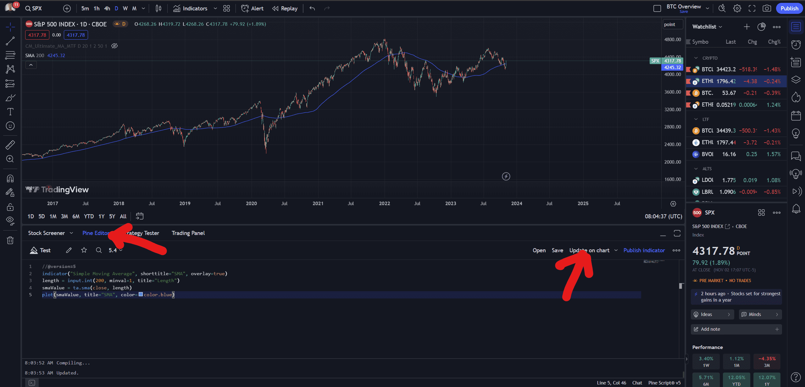
How To Add Pine Script To A Chart
To add this to a chart copy the code and paste it into the Pine Editor then click add to chart.
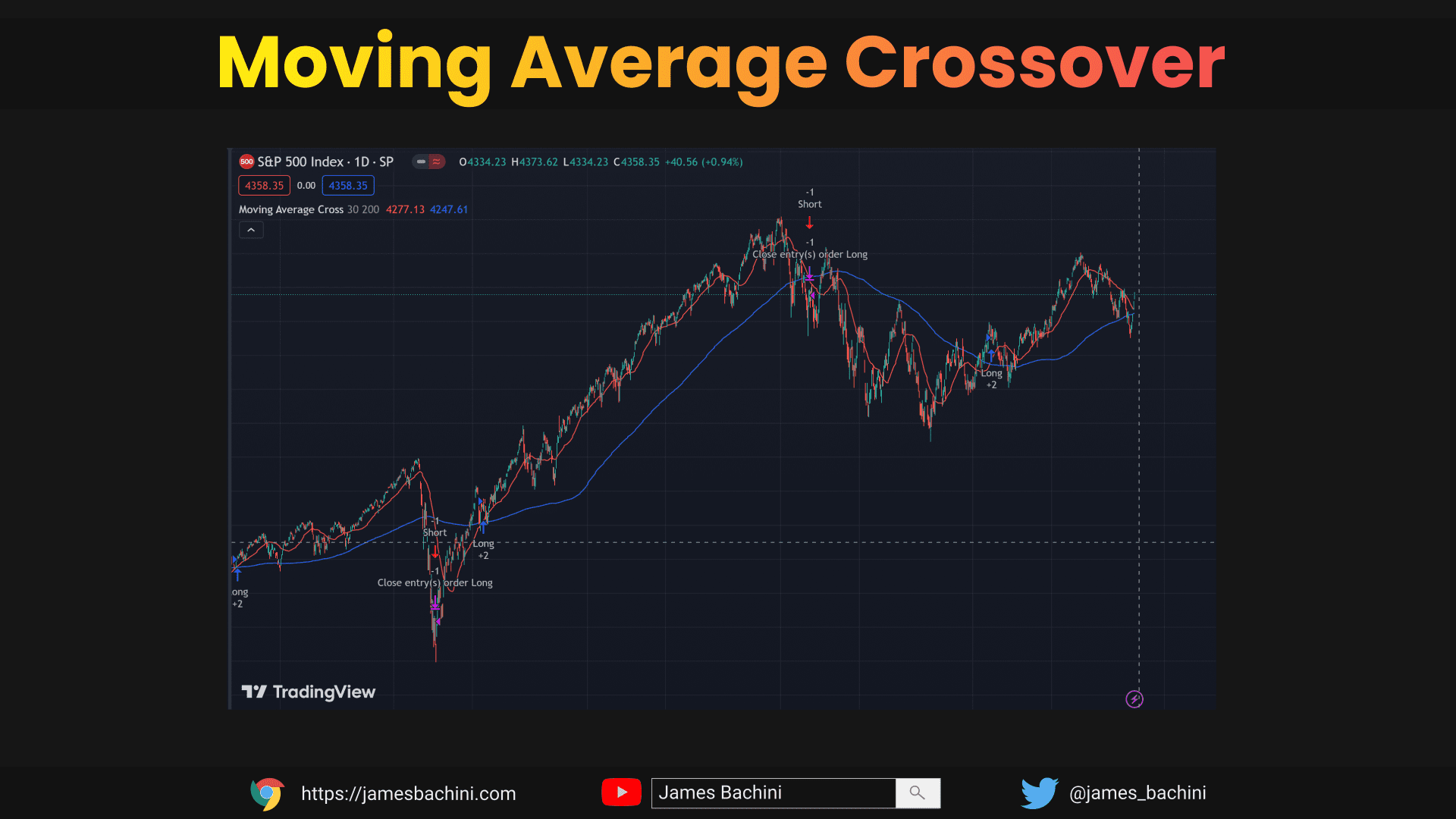
Creating A Strategy From An Indicator
In this example we are going to add a second simple moving average and create a trend following trading strategy. When the fast moving average crosses above the slow moving average we are long because price is going up, when the opposite is true we short.
https://github.com/jamesbachini/Pine-Script-Examples/blob/main/crossover.ps
//@version=6
strategy("Moving Average Cross", overlay=true)
shortLength = input.int(30, minval=1, title="Short Moving Average Length")
longLength = input.int(200, minval=1, title="Long Moving Average Length")
shortMA = ta.sma(close, shortLength)
longMA = ta.sma(close, longLength)
plot(shortMA, title="Short Moving Average", color=color.red)
plot(longMA, title="Long Moving Average", color=color.blue)
longCondition = ta.crossover(shortMA, longMA)
shortCondition = ta.crossunder(shortMA, longMA)
if (longCondition)
    strategy.entry("Long", strategy.long)
if (shortCondition)
    strategy.close("Long")
if (shortCondition)
    strategy.entry("Short", strategy.short)
if (longCondition)
    strategy.close("Short")
The first thing to note is that we declare our name and overlay as a strategy rather than an indicator on line 2.
Now let’s set the stage for our two main characters:
- shortMA – the short moving average with a default 30 period
- longMA – the long moving average with a default 200 period
We create user input settings for these with input.int and then use the ta.sma function to set the values, then we plot both lines on the chart using the plot function. All of this is done in the exact same way as the previous example.
We go on to define our conditions for making trades using the ta.crossover and ta.crossunder functions. The longCondition is a signal that springs into action when the shortMA line leaps over the longMA, suggesting the market’s heating up and it might be time to jump in. Conversely, the shortCondition is our lookout for when shortMA dips below longMA, hinting that things might be cooling down and there’s more potential downside.
Our script then puts these signals into action with the strategy.entry and strategy.close functions. When the crossover happens, it’s like a green light saying “Go long,” and when the crossunder occurs, it’s a red light indicating “Stop the long and go short”.
Backtesting Pine Script Strategies
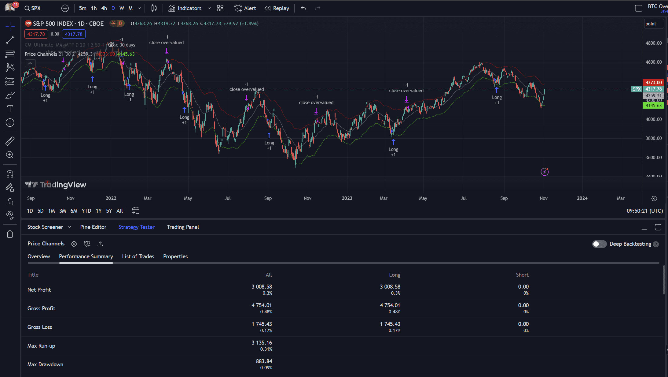
This is what I call a flip/flap strategy that switches long to short based on market conditions but always holds some directional position. Let’s see what it looks like on a chart.
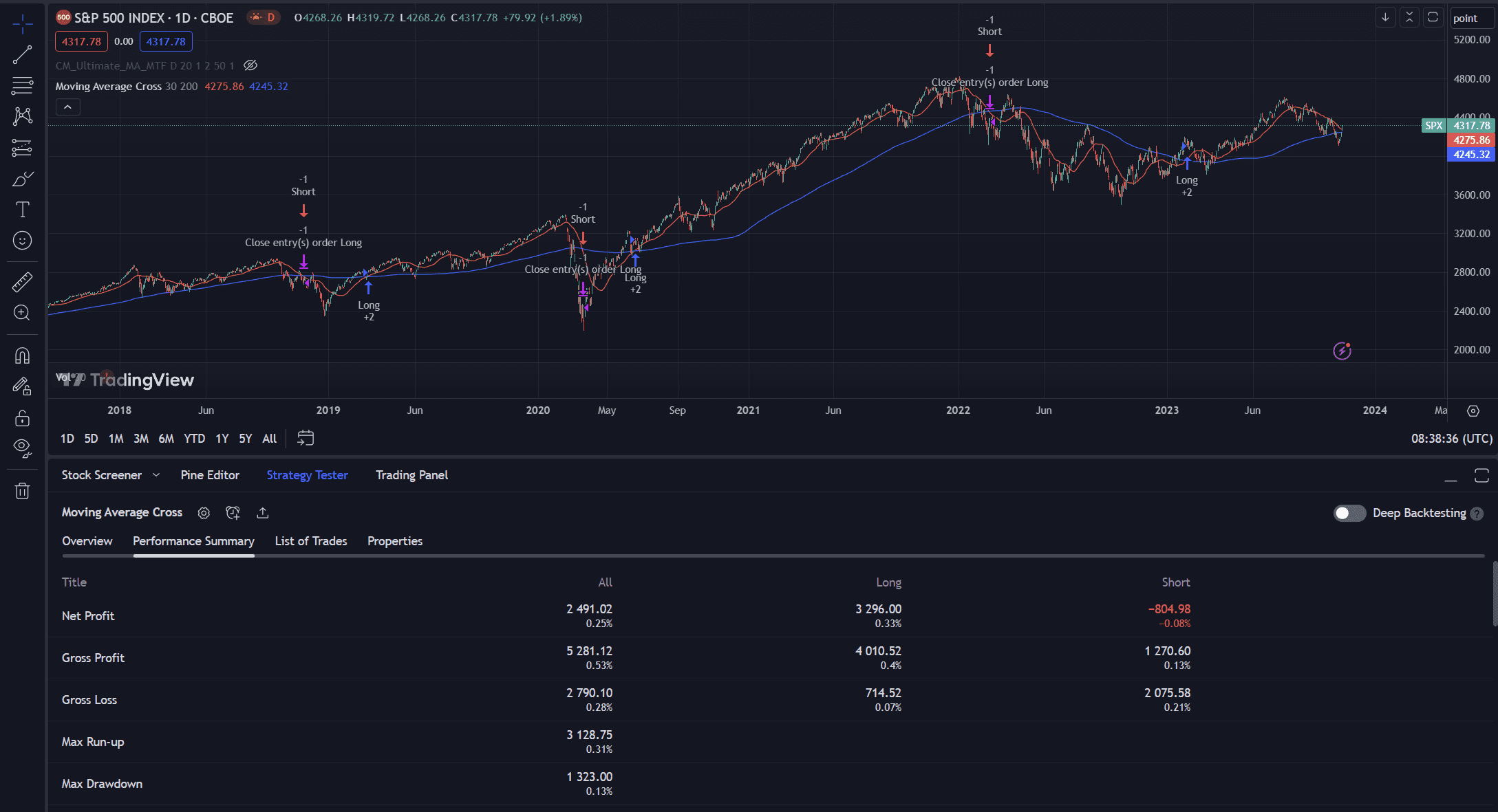
If we go into the next tab Strategy Tester (shown above) we can get backtesting metrics for how this has performed in the past based on historical data.
Notice that this simple trend following strategy on the daily S&P500 is more or less break even in a market that is up only over many decades. We could adjust the moving averages to find values where profits grow but we then risk over fitting our model.
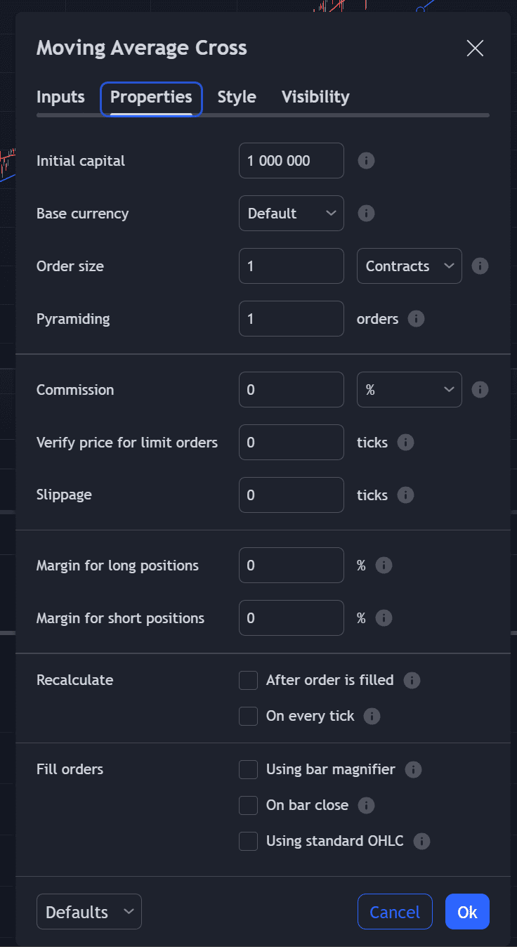
These backtests also aren’t perfect as we haven’t set any allowances for slippage, trading fees etc. While we can manually code these values into Pine Script I prefer to use the default settings in the properties tab which are available for every strategy.
Identifying Price Channels For Scaling In To A Position
Let’s say we have an asset that we want to buy into over a period of time. We could dollar cost average in or use a vwap bot or we could try and calculate fair value and then bid when price is at the extremities of good value.
To achieve this we will use two of the cornerstones of technical analysis moving averages and average true range. The moving average we have used before with the only difference being I want to use an EMA exponential moving average to have it more reflexive. The ATR or average true range provides a measure of volatility and some indication to how far we can expect price to move away from this fair value.
https://github.com/jamesbachini/Pine-Script-Examples/blob/main/price_channels.ps
//@version=6
strategy("Price Channels", overlay=true)
fairvalue = input.int(21, 'Exponential Moving Average', minval=1)
hold = input.int(30, 'Holding Period', minval=1)
mult = input.float(2, 'Multiplier', minval=0.1, step = 0.1)
atr = ta.atr(14)
ma = ta.ema(close, fairvalue)

resistance = ma + (atr * mult)
support = ma - (atr * mult)

plot(ma, 'Average', color=#AAAAAA88)
plot(support, 'Support', color=#00DD0088)
plot(resistance, 'Resistance', color=#DD000088)

if ta.crossover(close, support)
    strategy.entry("Long", strategy.long)
if ta.barssince(ta.crossover(close, support)) > hold
    strategy.close("Long", comment="close 30 days")
if ta.crossover(close, resistance)
    strategy.close("Long", comment="close overvalued")
We start by setting up a strategy and defining some inputs for the moving average period, max holding period of a trade and a multiplier which will define how far outside our fair value range we need price to go before we enter a trade.
Note that for the multiplier we are defining a input.float rather than an integer which means we can use decimal values. We also set the step increments to 0.1 so that this is reflected in the settings when the user clicks up or down.
We then calculate support and resistance bands using the moving average +- the atr * multiplier. This will give us a Bollinger band type indicator which looks a lot better on a chart than it does in a back test.
We plot all three lines on the chart for fair value (ema), support and resistance. One thing to note here is the color’s that I’m defining as RGBA (red, green, blue, alpha) values. There’s a nice color picker here if you want to create your own style.
Finally we set up the trade entry and two trade closes. The strategy will enter a trade when price goes below the support line. The trade will close when price goes above resistance or 30 days has passed since it last went below support.
We have a marginally profitable long strategy and we’ve identified areas where price is below fair value which is useful when entering long term positions over a period of time.
Building A Breakout Sniper
A breakout is when price breaks above a previous range high. With volatile assets this can often create high volatility trading opportunities. Let’s look at a strategy to identify and backtest a breakout sniper bot using Pine Script.
https://github.com/jamesbachini/Pine-Script-Examples/blob/main/breakout_sniper.ps
//@version=6
strategy("Breakout Sniper", overlay=true)
lookback_period = input.int(365, "Lookback Period", minval=1)
hold = input.int(30, 'Holding Period', minval=1)

highest_high = ta.highest(high, lookback_period)
lowest_low = ta.lowest(low, lookback_period)

plot(highest_high, 'HIGH', color=#CC000088)
plot(lowest_low, 'HIGH', color=#00CC0088)

breakout = high >= highest_high
breakdown = low <= lowest_low

if (breakout)
    strategy.entry("Long", strategy.long)
if ta.barssince(breakout) > hold
    strategy.close("Long", comment="close long")
if (breakdown)
    strategy.entry("Short", strategy.short)
if ta.barssince(breakdown) > hold
    strategy.close("Short", comment="close short")
We start by setting a look back period which we use to define the range high and low for that period using the ta.highest and ta.lowest technical analysis functions. We plot these on the chart to have some pretty lines and make it look like we know what we are doing.
Next we define a breakout when price is at the high for the lookback period and a breakdown when price is at the low for the same timeframe.
If price is breaking out we bid and go long, if price is breaking down we short it. In both cases we hold for 30 days and close the position.
Spoiler alert, trading breakouts on the SPX which tends to mean revert within a channel isn’t much fun but if we put it on a more volatile asset like Bitcoin…
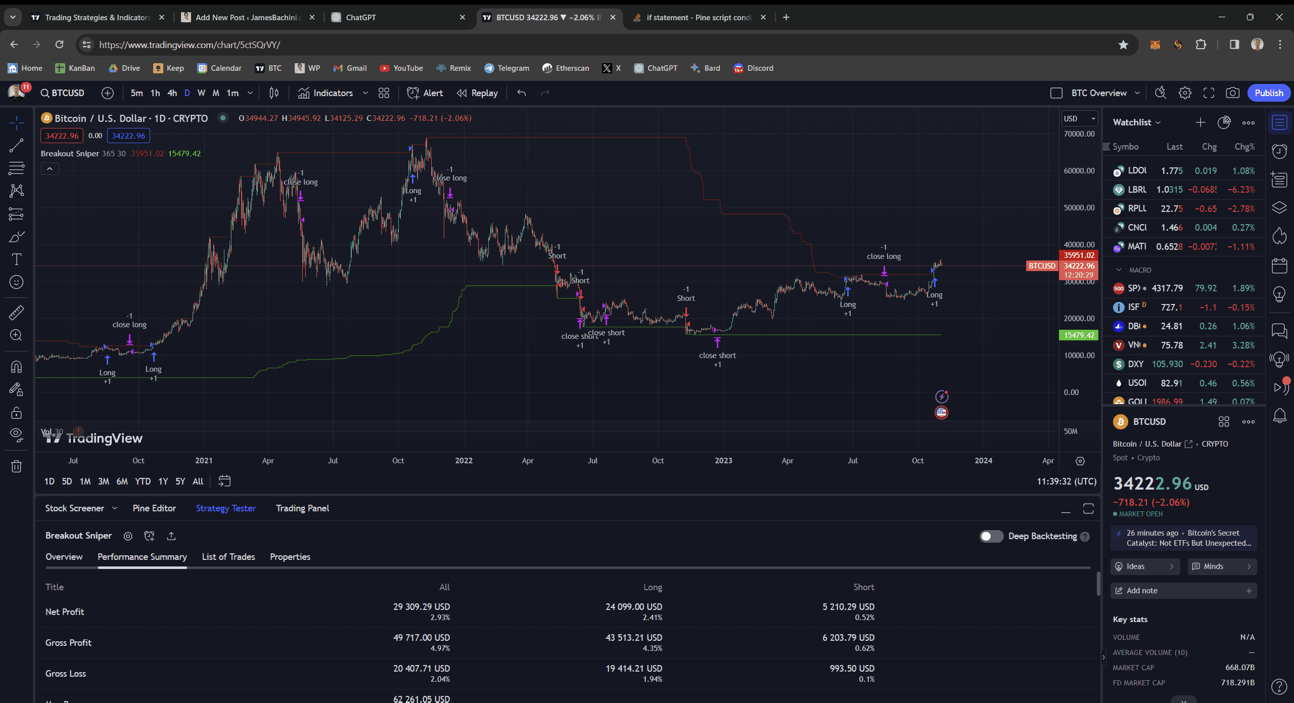
You can see we are making money on both the long and short side. The catch is that as digital asset markets mature I’d expect volatility to decrease and mean revert more often leading to more fakeouts and lower returns in the future. Having said that there are plenty of assets in tradfi and defi where you can find rampant speculation and volatility which are the foundations of a good breakout strategy.
Building A Fear/Greed Index
In the next example we are building an indicator which uses multiple data points to create a “fear and greed index“. This will be overlayed on the chart to highlight areas of extremes where markets have become irrational.
https://github.com/jamesbachini/Pine-Script-Examples/blob/main/fear_greed.ps
//@version=6
indicator("Fear and Greed Index", shorttitle="FGI", overlay=true)
extreme_fear = input.int(-40, "Extreme Fear")
extreme_greed = input.int(100, "Extreme Greed")
rsi = ta.rsi(close, 14)
fair_value = ta.ema(close, 14)
fv_indicator = (close / fair_value)
vol_high = ta.highest(volume, 90)
vol_low = ta.lowest(volume, 90)
vol_indicator = 1 + (volume / ((vol_high + vol_low) / 2))
stdev = ta.stdev(close, 14)
stdev_indicator = 1 + (stdev / close)
fgi = (rsi - 50) * fv_indicator * vol_indicator * stdev_indicator
bgcolor(fgi <= extreme_fear ? color.new(color.red, 90) : na)
bgcolor(fgi >= extreme_greed ? color.new(color.lime, 90) : na)
We are using RSI (relative strength index) as a starting point which is an oscillating indicator that ranges from 0-100.
We then create a fair value indicator using the close divided by the 14ema
We create a volume indicator using the current volume compared to high and low over a period of 90 days (or whatever timeframe the chart is set at).
Finally there is a volatility indicator using standard deviation.
We combine these indicators with a formula to create our fear and greed index
fgi = (rsi - 50) * fv_indicator * vol_indicator * stdev_indicatorAt the user defined extremities of the range we plot semi-transparent vertical line in either red for fear and green greed using the bgcolor and the color.new(color, transparency) functions.
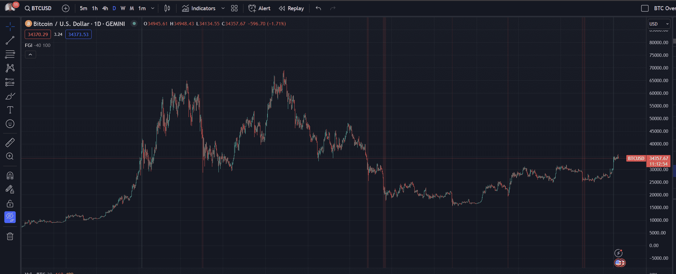
What we end up with is a indicator that can be placed on a chart to show times where price, volume and volatility are reaching extremes.
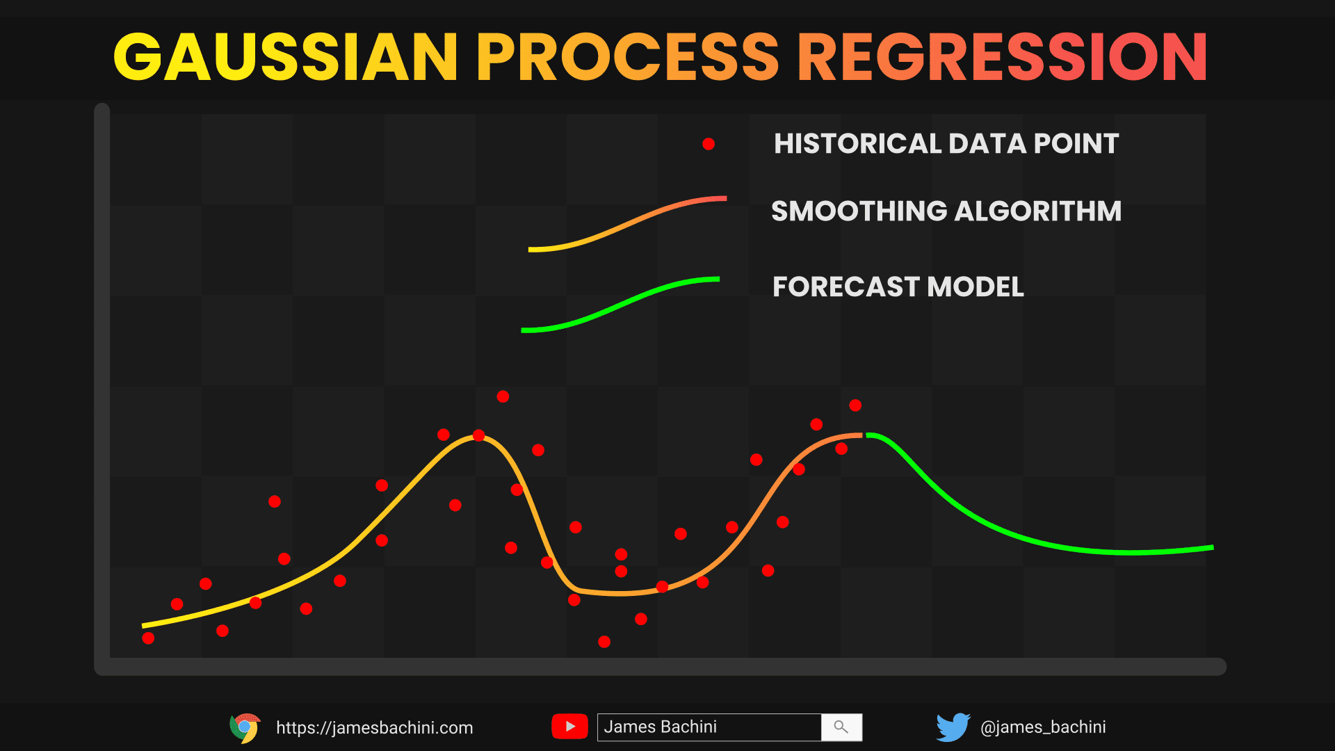
Gaussian Process Regression
Up until now we have mainly focused on lagging indicators and now it’s time to take on the somewhat impossible task of trying to predict the future.
Gaussian Process Regression (GPR), is a probabilistic modeling technique used to predict the likely future values of time series data. This approach is particularly useful for forecasting scenarios where the historical data is noisy and the relationships between values are complex and non-linear.
https://github.com/jamesbachini/Pine-Script-Examples/blob/main/gaussian_regression.ps
//@version=6
indicator("Gaussian Process Regression", shorttitle="GPR", overlay = true, max_lines_count = 300)
lookback_period = input.int(100, 'Lookback Period', minval=0)
prediction_horizon = input.int(30, 'Prediction Horizon', minval=0)
length_scale = input.float(10., 'Length Scale', minval=1)
noise_variance = input.float(0.1, step = 0.01, minval = 0)

radial_basis_function(x1, x2, scale) => math.exp(-math.pow(x1 - x2, 2) / (2.0 * math.pow(scale, 2)))

// Create a kernel matrix using the Radial Basis Function
create_kernel_matrix(training_set, test_set, scale) =>
    kernel_matrix = matrix.new<float>(training_set.size(), test_set.size())
    row_index = 0
    for train_point in training_set
        col_index = 0
        for test_point in test_set
            kernel_value = radial_basis_function(train_point, test_point, scale)
            kernel_matrix.set(row_index, col_index, kernel_value)
            col_index += 1
        row_index += 1
    kernel_matrix

var identity_matrix = matrix.new<int>(lookback_period, lookback_period, 0)
var matrix<float> prediction_kernel = na

// Set up initial training and test indices, noise matrix & compute the prediction kernel
if barstate.isfirst
    training_indices = array.new<int>(0)
    test_indices = array.new<int>(0)
    for i = 0 to lookback_period-1
        for j = 0 to lookback_period-1
            identity_matrix.set(i, j, i == j ? 1 : 0)
        training_indices.push(i)
    for i = 0 to lookback_period+prediction_horizon-1
        test_indices.push(i)
    noise_matrix = identity_matrix.mult(noise_variance * noise_variance)
    training_kernel = create_kernel_matrix(training_indices, training_indices, length_scale).sum(noise_matrix)
    training_kernel_inv = training_kernel.pinv()
    cross_kernel = create_kernel_matrix(training_indices, test_indices, length_scale)
    prediction_kernel := cross_kernel.transpose().mult(training_kernel_inv)

// Prepare the training outputs by subtracting the moving average from the close price.
current_index = bar_index
moving_average = ta.sma(close, lookback_period)
training_outputs = array.new<float>(0)
for i = 0 to lookback_period-1
    training_outputs.unshift(close[i] - moving_average)
predicted_means = prediction_kernel.mult(training_outputs)

// Loop through the predicted means to determine regression and forecast points
index_offset = -lookback_period+2
regression_points = array.new<chart.point>(0)
forecast_points = array.new<chart.point>(0)
for predicted_mean in predicted_means
    if index_offset == 1
        forecast_points.push(chart.point.from_index(current_index+index_offset, predicted_mean + moving_average))
        regression_points.push(chart.point.from_index(current_index+index_offset, predicted_mean + moving_average))
    else if index_offset > 1
        forecast_points.push(chart.point.from_index(current_index+index_offset, predicted_mean + moving_average))
    else
        regression_points.push(chart.point.from_index(current_index+index_offset, predicted_mean + moving_average))
    index_offset += 1
polyline.delete(polyline.new(regression_points, line_color = #FF00FF88, line_width = 10)[1])
polyline.delete(polyline.new(forecast_points, line_color = #FFFF0088, line_width = 10)[1])
The code is significantly more complex than what we have looked at so far so let’s break it down and into the major components.
- Initialization: The code defines the GPR indicator with customizable inputs for the lookback period, prediction horizon, length scale, and noise variance. These inputs allow users to adjust the sensitivity and behavior of the GPR based on their data.
- Kernel Function: A radial basis function (RBF) is defined, which is a commonly used kernel in Gaussian Process Regression. The RBF will be used to measure the similarity between different data points.
- Kernel Matrix Creation: create a kernel matrix that represents the relationships between training and test data points using the RBF. This matrix is central to the GPR method as it encapsulates the covariances between data points.
- Training and Prediction Setup: On the first bar of data, the code sets up the training and test indices, creates an identity matrix scaled by noise variance, and computes a prediction kernel. The prediction kernel is a transformation matrix that relates past observations to future predictions.
- Data Processing: The script calculates a moving average of the closing prices over the lookback period and prepares the training outputs by subtracting this moving average from the actual closing prices.
- Prediction Computation: Then we multiply the prediction kernel with the training outputs to produce predicted means. These are the GPR’s forecasts for future price movements.
- Drawing Predictions: Finally, the predicted means are used to generate two sets of points for plotting on the chart: regression points (for fitting to past data in pink) and forecast points (for predicting future data in yellow).
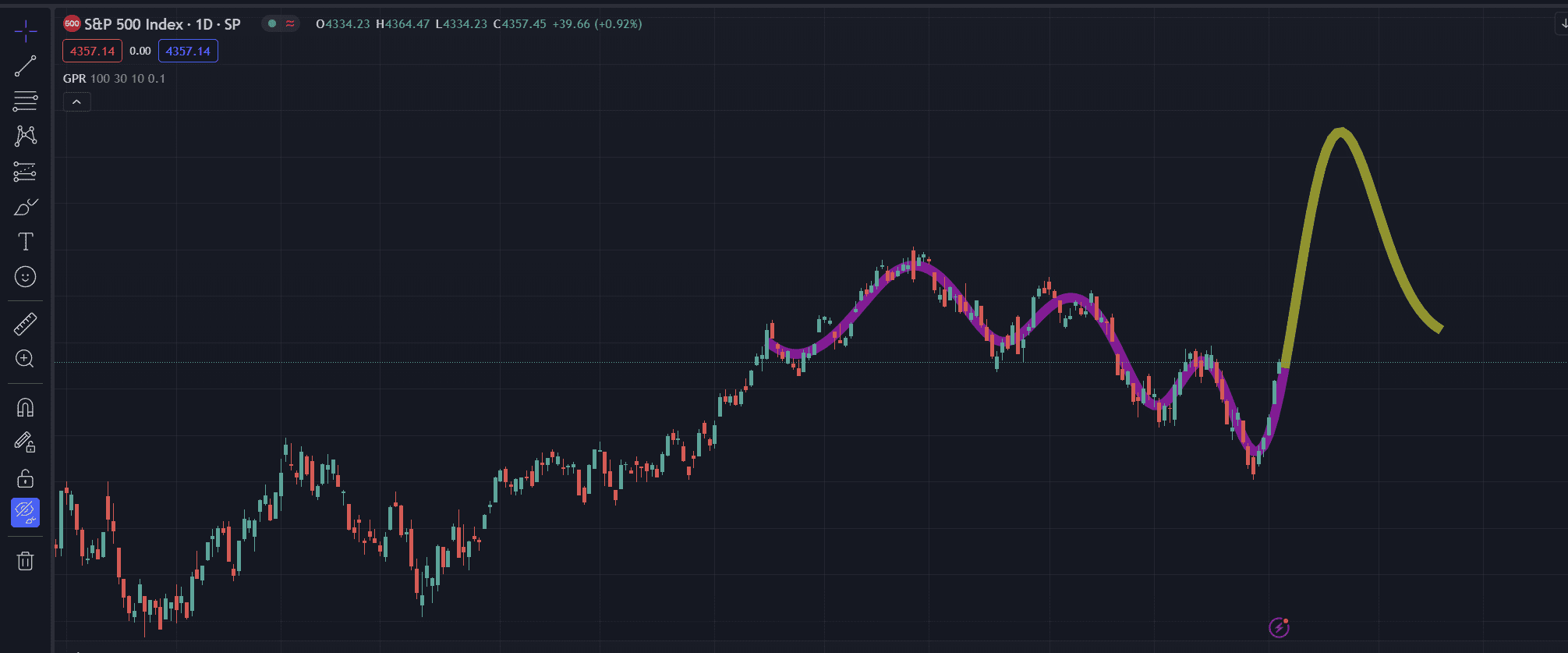
GPR is widely used throughout quantitative trading to forecast future price movements by modeling past price data. The method applies a kernel method to understand the data’s structure, and uses this information to make predictions. It’s by no means a magic crystal ball but is a useful indicator which provides valuable modelling for system traders.
I hope these examples have given you some ideas as to how you can craft your own unique indicators and strategies using Pine Script. If you want to learn more about trading digital assets I have a free newsletter at https://bachini.substack.com
